Young’s modulus computation
The computation of the Young’s modulus uses a look-up table (LUT) that was derived from simulations based on the finite elements method (FEM) [Mokbel2017] and the analytical solution [Mietke2015]. The LUT was generated with an incompressible (Poisson’s ratio of 0.5) linear elastic sphere model (an artificial viscosity was added to avoid division-by-zero errors) in an axis-symmetric channel (2D). Although the simulations were carried out in this cylindrical symmetry, they can be mapped onto a square cross-sectional channel by adjusting the channel radius to approximately match the desired flow profile. This was done with the spatial scaling factor 1.094 (see also supplement S3 in [Mietke2015]). The original data used to generate the LUT are available on figshare [FigshareWittwer2020].
The computations take into account scale conversions (channel width, flow rate) [Mietke2015], pixelation effects for deformation [Herold2017], and shear-thinning (for CellCarrier media) [Herold2017].
Since the Young’s modulus is model-dependent, it is not made available right away as an ancillary feature (in contrast to e.g. event volume or average event brightness).
In [1]: import dclab

In [2]: ds = dclab.new_dataset("data/example.rtdc")

# "False", because we have not set any additional information.
In [3]: "emodulus" in ds
Out[3]: False
Additional information is required. There are three scenarios:
- The viscosity/Young’s modulus is computed individually from the chip temperature for each event. Required information:
- The temp feature which holds the chip temperature of each event
- The configuration key [calculation]: ‘emodulus medium’
- The configuration key [calculation]: ‘emodulus model’
- Set a global viscosity. Use this if you have measured the viscosity of your medium (and know all there is to know about shear thinning [Herold2017]). Required information:
- The configuration key [calculation]: ‘emodulus model’
- The configuration key [calculation]: ‘emodulus viscosity’
- Compute the Young’s modulus using the viscosities of known media.
- The configuration key [calculation]: ‘emodulus medium’
- The configuration key [calculation]: ‘emodulus model’
- The configuration key [calculation]: ‘emodulus temperature’
Note that if ‘emodulus temperature’ is given, then this temperature is used, even if the temp feature exists (scenario A).
The key ‘emodulus model’ currently (2019) only supports the value
‘elastic sphere’. The key ‘emodulus medium’ must be one of the
supported media defined in
dclab.features.emodulus.viscosity.KNOWN_MEDIA and can be
taken from [setup]: ‘medium’.
The key ‘emodulus temperature’ is the mean chip temperature and
could possibly be available in [setup]: ‘temperature’.
import matplotlib.pylab as plt
import dclab
ds = dclab.new_dataset("data/example.rtdc")
# Add additional information. We cannot go for (A), because this example
# does not have the temperature feature (`"temp" not in ds`). We go for
# (C), because the beads were measured in a known medium.
ds.config["calculation"]["emodulus medium"] = ds.config["setup"]["medium"]
ds.config["calculation"]["emodulus model"] = "elastic sphere"
ds.config["calculation"]["emodulus temperature"] = 23.0 # a guess
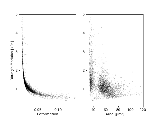
# Plot a few features
ax1 = plt.subplot(121)
ax1.plot(ds["deform"], ds["emodulus"], ".", color="k", markersize=1, alpha=.3)
ax1.set_ylim(0.1, 5)
ax1.set_xlim(0.005, 0.145)
ax1.set_xlabel(dclab.dfn.get_feature_label("deform"))
ax1.set_ylabel(dclab.dfn.get_feature_label("emodulus"))
ax2 = plt.subplot(122)
ax2.plot(ds["area_um"], ds["emodulus"], ".", color="k", markersize=1, alpha=.3)
ax2.set_ylim(0.1, 5)
ax2.set_xlim(30, 120)
ax2.set_xlabel(dclab.dfn.get_feature_label("area_um"))
plt.show()
(Source code, png, hires.png, pdf)
