Fluorescence traces
In RT-FDC, fluorescence data are stored alongside the regular image and scalar features. The fluorescence data consist of the trace data (fluorescence signal over time) and several scalar features (maximum, peak position, peak width, etc.) for each fluorescence channel. The trace data are stored as raw and median-filtered traces, where median-filtered means that the raw data is filtered with a rolling median filter.
In [1]: import dclab

In [2]: ds = dclab.new_dataset("data/example_traces.rtdc")

# list the available traces in the dataset
In [3]: sorted(ds["trace"].keys())
Out[3]: ['fl1_median', 'fl1_raw', 'fl2_median', 'fl2_raw', 'fl3_median', 'fl3_raw']

# show fluorescence meta data
In [4]: ds.config["fluorescence"]
Out[4]:
{'bit depth': 16,
 'channel 1 name': '525/50',
 'channel 2 name': '593/46',
 'channel 3 name': '700/75',
 'channel count': 3,
 'channels installed': 3,
 'laser 1 lambda': 488.0,
 'laser 1 power': 8.0,
 'laser 3 lambda': 640.0,
 'laser 3 power': 100.0,
 'laser count': 2,
 'lasers installed': 3,
 'sample rate': 312500.0,
 'samples per event': 177,
 'signal max': 1.0,
 'signal min': -1.0,
 'trace median': 0}
Please note that the value of trace median is zero (no median filter applied),
which tells us that the values of the raw and median trace data are identical.
The example dataset is an excerpt from the calibration beads dataset,
with a total of three fluorescence channels used.
import matplotlib.pylab as plt
import dclab
ds = dclab.new_dataset("data/example_traces.rtdc")
# event index to plot
idx = 8
# measuring time
samples = ds.config["fluorescence"]["samples per event"]
sample_rate = ds.config["fluorescence"]["sample rate"]
t = np.arange(samples) / sample_rate * 1e6
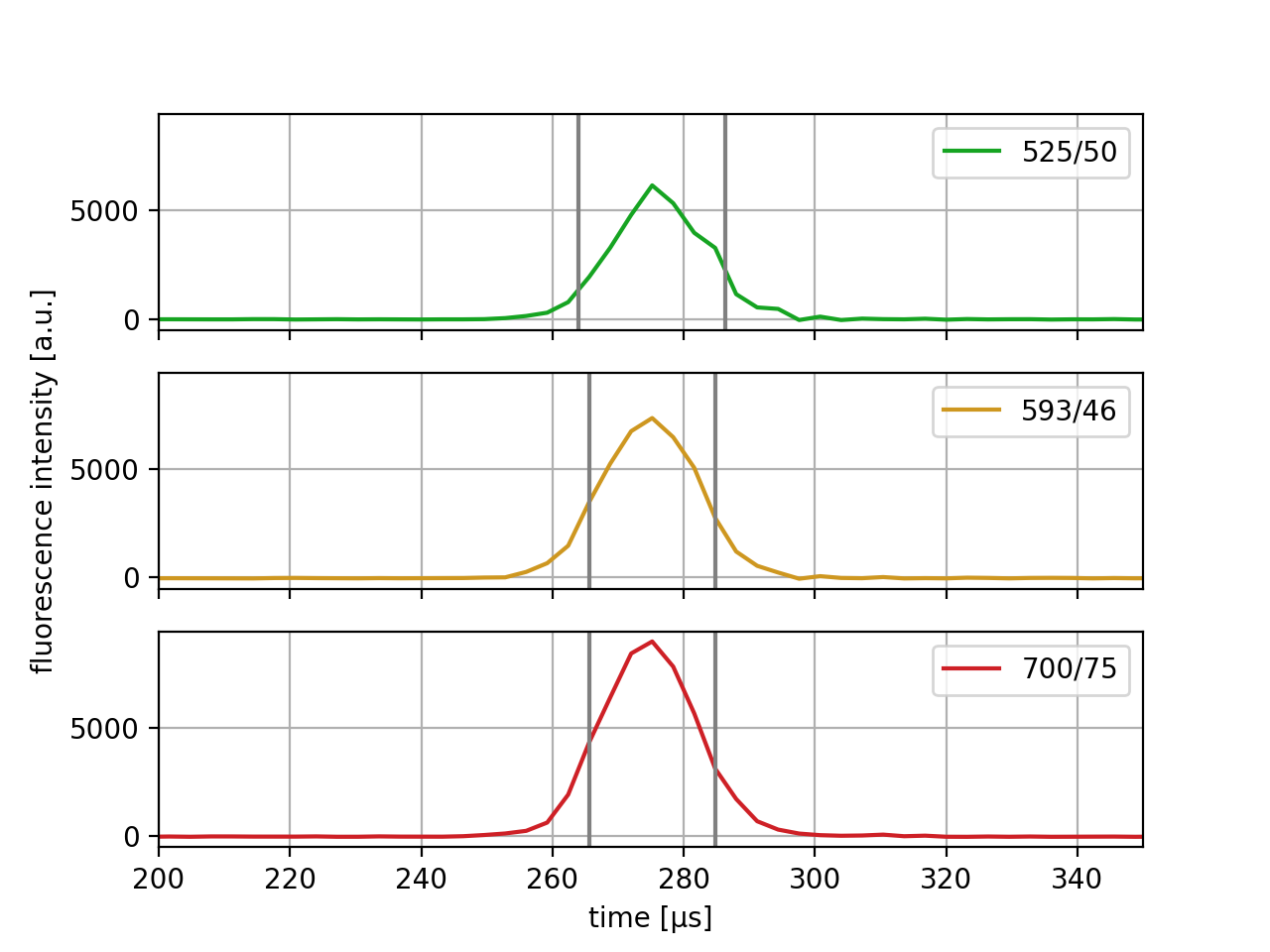
fig, axes = plt.subplots(nrows=3, sharex=True, sharey=True)
# fluorescence traces (colors manually chosen to represent filter set)
axes[0].plot(t, ds["trace"]["fl1_median"][idx], color="#16A422",
label=ds.config["fluorescence"]["channel 1 name"])
axes[1].plot(t, ds["trace"]["fl2_median"][idx], color="#CE9720",
label=ds.config["fluorescence"]["channel 2 name"])
axes[2].plot(t, ds["trace"]["fl3_median"][idx], color="#CE2026",
label=ds.config["fluorescence"]["channel 3 name"])
# detected peak widths
axes[0].axvline(ds["fl1_pos"][idx] + ds["fl1_width"][idx]/2, color="gray")
axes[0].axvline(ds["fl1_pos"][idx] - ds["fl1_width"][idx]/2, color="gray")
axes[1].axvline(ds["fl2_pos"][idx] + ds["fl2_width"][idx]/2, color="gray")
axes[1].axvline(ds["fl2_pos"][idx] - ds["fl2_width"][idx]/2, color="gray")
axes[2].axvline(ds["fl3_pos"][idx] + ds["fl3_width"][idx]/2, color="gray")
axes[2].axvline(ds["fl3_pos"][idx] - ds["fl3_width"][idx]/2, color="gray")
# axes labels
axes[1].set_ylabel("fluorescence intensity [a.u.]")
axes[2].set_xlabel("time [µs]")
for ax in axes:
ax.set_xlim(200, 350)
ax.grid()
ax.legend()
plt.show()
(Source code, png, hires.png, pdf)

Please note that the fluorescence traces are stored as integer values
and have to be converted to µs using the meta data stored in
ds.config["fluorescence"]. Also, notice how the scalar features
are used for plotting the peak width.